heatmap.py: create heatmaps in python
Download: Linux, OSX heatmap-2.2.1.tar.gzDownload: Windows heatmap-2.2.1.zip
github: heatmap on github
To install:
$ cd heatmap-2.2.1; python setup.py installRequires the Python Imaging Library and Python 2.5+.
Example
import heatmap
import random

if __name__ == "__main__":
    pts = []
    for x in range(400):
        pts.append((random.random(), random.random() ))

    print "Processing %d points..." % len(pts)

    hm = heatmap.Heatmap()
    img = hm.heatmap(pts)
    img.save("classic.png")
Changelog
2.2.1 - 11 Jan 13 [tgz] [zip]- pip install bugfix. sorry pip folks! thanks to Jordi Llonch again for the bugfix
- bugfix in the area parameter for non-square areas; thanks to github.com/y3pp3r
- modifed API to return Image instance; caller must specify filename
- restructured project layout to be more standardized
- added to pypi
- many thanks to Jordi Llonch for the pull request
- added cygwin installation support, thanks to Michael C.
- fixed gross omission of kml support.
- fixed bug in minimum value computation with negative values
- fixed broken opacity for areas with no density
- fixed bug that flipped x/y coordinates - thanks to Curt Hartung for the find and fix
- added area parameter to allow caller to specify data bounds - thanks to Alex Little for the design.
- various small cleanups
- moved heavy lifting into C module. Compiles on POSIX systems, pre-compiled DLLs provided for x86 and x64 Windows systems. Significant perf increase: now 10k points in 5s
- joined the fad and moved source to github.
- modified _colorize() to not use putpixel; reduced processing time for 1024x1024 image from 14s to 5s for 100 points
- Initial release
Bugs, Feedback, Comments or Questions
@jjguyjjg@jjguy.com
github
Highlights
heatmap() takes a list of x, y coordinate tuples and returns a PIL Image object describing their density as a heatmap. Some highlights:
- Independent autoscaling in both x and y ranges
- Variable output image size
- Five output color schemes
- Tweakable intensity by modifying point size
- Google Earth KML output (assumes input coordinates are lat/long in decimal degrees)
Google Earth
After creating the output image, you can call saveKML() to create a KML file for Google Earth. It assumes the list of input points are a series of lat/long coordinates in decimal degrees. When loaded into Google Earth, you will see the heatmap as a Ground Overlay.
import heatmap
import random

hm = heatmap.Heatmap()
pts = [(random.uniform(-77.012, -77.050), random.uniform(38.888, 38.910)) for x in range(100)]
hm.heatmap(pts)
hm.saveKML("data.kml")
A heatmap over downtown Washington, DC:
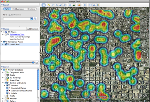
Heatmap loaded into Google Earth
1024x1024 image, opacity 128, 150px dotsize
100 random points in downtown DC
Color Schemes
heatmap() comes with 5 color schemes:
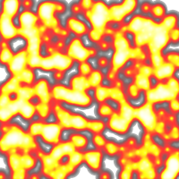
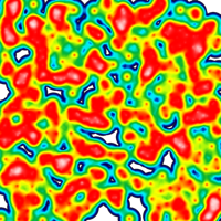
 classic |
 fire |
 omg |
 pbj |
 pgaitch |
|
|
Available color schemes Colors at the top are used for the densest areas, the bottom the sparsest. |
|||||
These color schemes are directly from gheat. (See 'credit', below) 'classic' is used by default, use another via the 'scheme' argument:
    hm = heatmap.Heatmap()
    hm.heatmap(pts, scheme='fire').save("fire.png")
Details
heatmap() has only two required parameters:
- A list of two-element tuples
- The filename to save the resulting image
 |  heatmap(self, points, dotsize=150, opacity=128, size=(1024, 1024), scheme='classic', area=None)
 |      points  -> an iteratable list of tuples, where the contents are the
 |                 x,y coordinates to plot. e.g., [(1, 1), (2, 2), (3, 3)]
 |      dotsize -> the size of a single coordinate in the output image in
 |                 pixels, default is 150px.  Tweak this parameter to adjust
 |                 the resulting heatmap.
 |      opacity -> the strength of a single coordiniate in the output image.
 |                 Tweak this parameter to adjust the resulting heatmap.
 |      size    -> tuple with the width, height in pixels of the output PNG
 |      scheme  -> Name of color scheme to use to color the output image.
 |                 Use schemes() to get list.  (images are in source distro)
 |      area    -> Specify bounding coordinates of the output image. Tuple of
 |                 tuples: ((minX, minY), (maxX, maxY)).  If None or unspecified,
 |                 these values are calculated based on the input data.
 |
 |      Returns a PIL Image object.  Call .save(fname) to write to disk.
Most options are self-explanatory, but dotsize, opacity and area could use some background.
Tweaking the heatmap output
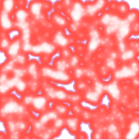
During processing, heatmap() builds a temporary image of one point. The image is grayscale, has radius of dotsize pixels and a decreasing density from the center outwards. A single dot at the default dotsize (150px) looks like this:

A single point
The dot is placed into the output image for each input point at the translated output image coordinate. The input points are unbounded. Values between 0 and 1 work as well as values between 5600 and 930000. The smallest points are placed at (0, 0) in the output image, with the largest points at (width, height). The x and y axes autoscale independently of each other.
Dots are blended into the output image with an additive process: as points are placed on top of each other, they become darker. After all input points have been blended into the output image, the ouput image is colored based on the darkness of each pixel.
Before colorization, the sample script above builds (in memory) an intermediate output image similar to:
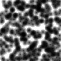
Before colorization
400 random points, 0 < pt < 1
1024x1024 image, 150px dotsize, opacity 255
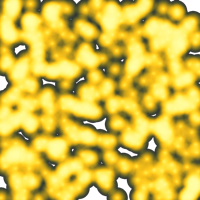
After colorizing with the 'classic' scheme (the default), the same image looks like this:
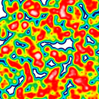
After colorization with the 'classic' scheme.
400 random points, 0 < pt < 1
1024x1024 image, 150px dotsize, opacity 255
Appropriate dotsize is a factor of your output image size, the density of your dataset and desired results. Tweak as you see fit.
Opacity changes the transparency of the color during the colorization process. If you want to use the heatmap as an overlay, set the opacity such that you get your desired results.
Autoscaling
Version 2.1 added the area parameter, to allow override of the autoscale functionality. The design follows Alex Little's design, described in his blog post Applying weighting to heatmaps.
The area parameter is a tuple of tuples: ((min x, min y), (max x, max y)). If the area parameter is specified, the (min x, min y) values will be associated with image pixels (0, 0); values (max x, max y) will be associated with image pixels (size x, size y), dependent on image output resolution.
For example, random.random() produces outputs between 0 and 1. To add a small border around the images, we can specify the area to be (-0.25, 1.25):
>>> import heatmap
>>> import random
>>> pts = [(random.random(), random.random()) for x in range(50)]
>>> hm = heatmap.Heatmap()
>>> hm.heatmap(pts, area=((-0.25, -0.25), (1.25, 1.25))).save("classic.png")
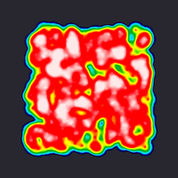
User-specified area
400 random points between 0 and 1
Area specified as -0.25 to 1.25 in both x and y
1024x1024 image, 150px dotsize, opacity 255
Feedback
This worked well enough for my datasets, but I had to tweak the algorithm several times. If it doesn't work for your data, send me feedback (and your source data, if you can.) I'll try to get more generalized algorithms in future releases.
Credit
The technique and color schemes came from gheat. If you need a web-enabled interface to heatmaps with Google Maps, gheat is a good tool for the job. I didn't do anything original, but merely took their work and generalized it. Chad credits the definitive heatmap as his starting point. Like those projects, this project is under the MIT license.